
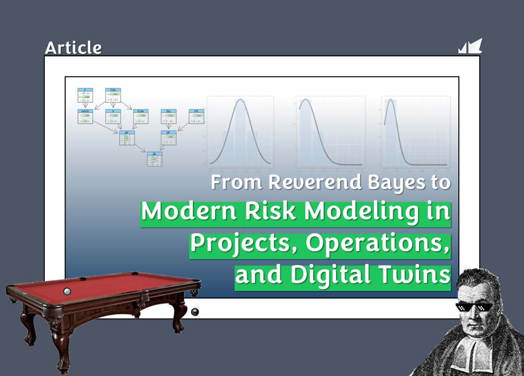
From Reverend Bayes to Modern Risk Modeling in Projects, Operations, and Digital Twins
Bayesian Methods for Risk Modeling - Part 1

Some might say Reverend Bayes was a bit obsessive. They wouldn’t be wrong.
It was his obsession, however, that nudged open the door to one of the universe’s most profound laws of reasoning.
What began as a quiet attempt to reason from effect back to cause would, centuries later, evolve into an entire framework for understanding complexity, risk, AI, and adaptive decision-making.
In this article, we begin with the early history of Bayes' theorem and trace its evolution to modern-day applications in risk modeling. We review:
What was wrong with Reverend Bayes?
Bayes’ Pool Table Thought Experiment
Mathematics of Risk
From Thomas Bayes to Bayesian Networks
Three Fundamental Patterns of Probabilistic Interdependence
Risk Modeling with Bayesian Networks
Bayesian Networks in Projects and Operations
Bayesian Networks in Digital Twins
Question then Becomes
Bayesian Networks (BNs), build on Bayes’ original insight by modeling the probabilistic dependencies between variables using directed acyclic graphs (DAGs). These networks capture how real-world phenomena influence one another, not through isolated causes, but through structured chains of probabilistic dependencies (1–4).
Over the years, Bayesian methods have proven to be powerful tools for tackling real-world challenges in projects and operations risk modeling, and systems engineering. This article is part of a course developed at the University of Calgary, focused on practical applications of Bayesian methods.
What was Wrong with Reverend Bayes?
From limited information we have, it appears that Reverend Thomas Bayes (1702–1761) was a quiet intellectual, driven by both religious faith and a rigorous sense of logic.
In his later years, he turned to a deceptively simple question: How should we update our beliefs in light of new information? Perhaps he recognized that the human brain does this instinctively, given wet sidewalks, we infer rain. But his goal was to mathematically determine the likelihood of a hidden cause given an observed effect.
Unlike classical probability, which predicts outcomes based on known conditions, Bayes sought to reverse the lens: to reason backwards from data to underlying causes.
Bayes, however, never articulated his findings using today’s formalism. After his death, Richard Price, his friend and colleague found an unfinished paper in his files titled An Essay Towards Solving a Problem in the Doctrine of Chances (1763). Realizing its importance, Price edited, completed, and prepared the work for publication. He also wrote an introduction to explain and contextualize the significance of Bayes’ result. The torch was later carried forward by Pierre-Simon Laplace, who extended Bayes’ ideas into a broader and more influential framework.
Bayes’ Pool Table Thought Experiment
Imagine a pool table stretching from 0 to 1m. Now let us consider the following three acts.
First - Somewhere along this table, a wooden bar is placed at a secret location, call it X. The exact position is hidden from us; all we know is that it's somewhere between 0 and 1, chosen uniformly at random. This unseen position represents a probability we want to uncover.
Second - A ball is dropped. But this one land according to a rule—it falls randomly somewhere between 0 and X, again chosen uniformly, call it Y.
Third Act – The wooden bar is removed. The only thing we can observe is Y.
And now the essential question arises: given this observed Y, what can we reasonably infer about the unknown X? In other words, how do we revise our belief about where the wooden bar might have been placed?

Engaging with the Experiment
First, the hidden value X—the location of the wooden bar—is assumed to be uniformly distributed between 0 and 1. This means, before observing anything, we treat all positions as equally likely.
Second, the observed value Y, the landing spot of the ball, and we know is also uniformly distributed over the interval between 0 and X. So once X is fixed (though unknown to us), Y is equally likely to land anywhere from 0 up to that value.
When we observe Y, one thing becomes immediately clear: the unknown value X must be greater than Y. The ball couldn’t have landed outside the range from 0 to X, so Y < X.
But beyond that, something more subtle happens. We can reason those smaller values of X—those just slightly larger than Y—are more likely than much larger ones. Why? Because for Y to have landed near itself within a large interval (say from 0 to 0.9), it would have to be a rather rare, although not impossible, outcome.
This asymmetry shifts our belief. After seeing Y, we no longer consider all values of X equally likely. We now prefer those that are closer to Y, while still greater than it. In Bayesian terms, we’ve updated our prior belief (from X uniformly distributed between 0 and 1) into a posterior belief—one that leans toward values of X just above the observed Y.
What we now call Bayes’ rule—or Bayes’ theorem—is a direct consequence of the basic rule of conditional probability that Reverend Thomas Bayes used to calculate the probability of a hidden cause X, given an observed outcome Y, also known as the Posterior distribution of P(X|Y).
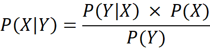
In the context of the table and ball experiment, applying Bayes’ rule for values where X > Y leads to a specific form of the posterior distribution that is shown in Figure 2.
For example, let’s say Y = 0.3. Before observing anything, we assume X follows a uniform distribution between 0 and 1—represented as the red line in Figure 1. But after seeing Y = 0.3, the updated belief (the blue curve) tilts in favor of values just above 0.3. As expected, smaller values of X closer to 0.3 are now more probable than those closer to 1.
Importantly, the area under the posterior curve still sums to 1, preserving the total probability. What changes is not the amount of belief, but how that belief is distributed.
 is uniform, while the posterior P(X∣Y=0.3) favors lower values of X, illustrating Bayesian updating.")
In the decades following Bayes’ quiet mathematical insight, it was Pierre-Simon Laplace who expanded this modest idea into a grand framework for reasoning under uncertainty. Between 1774 and 1812, Laplace independently developed and generalized what we now call Bayesian probability.
Laplace introduced the formal concepts of prior (here P(X)), and posterior (probability, giving structure to the idea of updating beliefs in light of new data. He was also the first to express Bayes’ Theorem in its modern algebraic form and apply it rigorously to real-world problems, particularly in astronomy and statistical estimation.
Inverting Probabilities, Updating Beliefs
Bayes’ rule has become the fundamental mathematics of probabilities and an indispensable part of risk modeling. It helps us update what we believe based on what we observe.
For example, if you’re vaccinated and want to know the chance, you’ll still get a disease, Bayes’ rule lets you calculate that by inverting data of how many vaccinated people got sick.

This same approach is central to Bayesian statistics. In traditional (frequentist) statistics, we usually start with a model and ask: If this model is true, how likely is it that we would observe this data? This is useful, but it doesn’t directly tell us how confident we should be in the model itself.
Bayesian statistics inverts this proposition. Using Bayes’ rule, we ask: Given the data we've observed, how likely is it that this model is true? Instead of just asking how likely the data are under a given model? Bayes rules allow us to answer given the data, how likely is the model?

This shift is powerful. It means we can compare different models or hypotheses directly, update our confidence in them as new data arrives. It turns statistics into an evolving dialogue between belief and evidence. We will delve deep into Bayesian statistics in the second part of the course.
From Reverend Bayes to Bayesian Networks
Once we understand the relationship between X and Y, the natural next step can be to follow the chain further: what about a third variable, or a fourth?
If the table and ball experiment taught us how to infer X from Y, we can imagine continuing the sequence. Suppose we now place a wooden bar at position Y, and drop a second ball that lands somewhere position Z < Y. This gives us a new question: Given Z, what can we say about Y? And in turn, what does that tell us about X?

This idea of connected, conditional relationships, where knowledge flows from one variable to another, laid the foundation for connecting large networks of variables in what is known now as Bayesian Networks.
Bayesian Networks
While several scholars had continued exploring this idea, including the notable Professor Andrey Markov in the early 20th century, the formal foundation of Bayesian Networks was proposed more recently, in the 1980s, by Judea Pearl.
Pearl transformed Bayes’ rule from a two-variable equation into a framework for reasoning across entire webs of interconnected uncertainty. In his book, Probabilistic Reasoning in Intelligent Systems (1988), Pearl introduced Bayesian Networks as graphical models that use directed acyclic graphs (DAGs), as shown in Figure 4, to represent dependencies among variables (5).
")
In his recent research biography, The Book of Why, Pearl suggests that he drew inspiration for message passing through layers and nodes from early advances in neural networks (3).
Pearl, along with other key scholars, played a central role in advancing inference in Bayesian Networks through the development of belief propagation, also known as message passing. This method made it possible to perform efficient probabilistic inference, even in complex systems with many interdependent variables.
Building on this foundation, Philip Dawid (1992) formalized the clique tree representation, which provided a structured way to organize computations across interconnected variables(6). Ross D. Shachter (1986) introduced the tree decomposition method for exact inference, enabling networks to be restructured into simpler forms suitable for computation (7). In a key advance, Steffen Lauritzen and David Spiegelhalter (1988) applied the junction tree framework to Bayesian inference, allowing for local computations instead of costly global ones(8). Finally, Finn Jensen (1994) contributed by developing practical implementations of the algorithm, helping bring these theoretical advances into widespread use (9).
Wider Adoption and Impact
By the 1990s, Bayesian Networks had found their place in AI, expert systems, and decision-support tools.
Microsoft, for instance, used them in its Office troubleshooting assistant. The networks enabled machines to reason in uncertain environments, just as humans do—by updating beliefs, weighing alternatives, and inferring hidden causes from visible effects.
In a 1990s Los Angeles Times article, Bill Gates, then Microsoft Chairman, stated that Microsoft's competitive advantage, particularly in areas like understanding human speech and building internet services, was its expertise in "Bayesian networks".
“Microsoft's competitive advantage is its expertise in Bayesian networks.”
- Bill Gates, 1990
From a single hidden ball on a table to vast networks modeling disease, risk, or intent, the journey from Bayes’ rule to Bayesian Networks reveals a deep truth: knowledge doesn't exist in isolation—it spreads through structured, conditional relationships. The real power lies in tracing those threads.
Three Fundamental Patterns of Probabilistic Interdependence
As we expand from two to three variables, a new layer of complexity emerges.
There are only three distinct ways to structure three nodes in a directed acyclic graph (DAG), each with a different pattern of causal influence. These three configurations, shown in Figure 5, form the fundamental building blocks of all Bayesian Networks(1).
 a chain where A causes B and B causes C, labeled as \"Cause and Effect,\" (2) a fork where A causes both B and C, labeled as \"Common Cause,\" and (3) a collider where A and B both cause C, labeled as \"Common Effect.\" These structures represent the core building blocks of Bayesian networks and illustrate different types of probabilistic interdependence.")
The first structure is the sequential chain (Figure 5) where A affects C through mediator B. Therefore, conditioned on B, A and C are independent. For example, remoteness, affects the need for new infrastructure, which in turn affects cost. By knowing the exact need for infrastructures, remoteness becomes independent of cost (through that pathway).
The diverging structure in Figure 5 is the declaration of a common cause. The C and B are probabilistically dependent through A, and independently conditioned on A. For example, remoteness, affects the need for new infrastructure, and through another pathway, it affects the labor shortage. In absence of knowledge about the project’s remoteness, it is possible to “induce” that a project with labor shortage, may as well require more infrastructure spending, as it may be remote. However, knowing the degree of remoteness blocks this dependency by creating a conditional independence. Therefore, labour shortage is independent of infrastructure spending when the remoteness is already known. This form of inductive reasoning allows for modeling the latent risk factor (i.e., risk driver) through their effects on measurable risk indicators.
The converging structure in Figure 5 is the declaration of a common effect. The structure exerts that A, and B are probabilistically independent, but both affect C. However, conditioning on C creates probabilistic dependency between A and B. For example, the project profitability is a common effect of both the payback period, and the rate of return. In the absence of knowledge about profitability, the payback period and the rate of return are independent. However, knowing that the project is not profitable creates a conditional dependence between the two. If the rate of return is high, the low profitability of the project can only be explained away by a long and undesirable payback period. Unlike the previous two structures where conditioning on the cause or the mediator creates probabilistic independence, conditioning here on the effect creates dependence.
Together, these three structures—chains, forks, and colliders—are the DNA of Bayesian reasoning. They show how causality, dependence, and inference can shift dramatically depending on where in the network we look—and what we condition on.
Mathematics of Risk
In many instances, risk can be a qualitative and multi-faceted concept, it may involve social judgment, ethical concerns, and strategic trade-offs.
However, when we need to quantify risk for decision-making and modeling, we can break it down into three core elements: a scenario or event that might occur, the likelihood of that event, and the consequence if it happens.
This decomposition gives us the classic risk triplet:
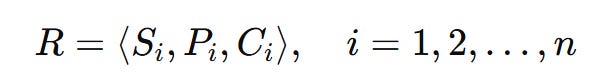
Si: a specific scenario or set of events that leads to exposure or harm
Pi: the likelihood or frequency of that scenario
Ci: the consequence, such as financial loss or operational impact
To assess whether these consequences matter, we introduce another layer: thresholds, denoted Tj. These are the limits of acceptable impact across different domains, 1 to j, such as finance, safety, environment, or reputation. A risk becomes significant, to various degrees, when the expected consequence Pi Ci exceeds a relevant threshold Tj.
At a preliminary maturity level in risk modeling, we might treat the likelihood Pi as a fixed probability, and the consequence, Ci, and the threshold, Tj, as deterministic values (single numbers).
At higher maturity levels, we recognize that all three elements—likelihood, consequence, and threshold—carry uncertainty. These are not always known with precision; they often depend on expert judgment, assumptions, or incomplete and scarce previous data.
Just like the position of the first and second balls on the pool table, Z, and Y, inform us about the uncertainty of the location of the disappeared wooden bar, X. Bayesian methods allow us to work with uncertainties at both levels.
Bayesian methods provide a mathematical framework that allows for two fundamental reasoning capabilities.
To model real world phenomena as part of connected systems with probabilistic interdependencies, and,
to represent our current understanding and expert judgement as probability distributions and update them as new evidence and data emerges.
Risk Modeling with Bayesian Networks
The classic bow-tie diagrams are useful conceptualizations of risk.
As shown in Figure 6, the bow-tie diagram illustrates a hazardous event at the center, flanked by causes on the left and consequences on the right. It helps visualize how threats may lead to loss of control, and how recovery measures can mitigate consequences.

In conventional risk and reliability engineering, this conceptual bow-tie is often transposed into a combination of Fault Tree Analysis (FTA) and Event Tree Analysis (ETA), as seen in Figure 7. FTA traces backward from a system failure to its root causes through logical gates, while ETA projects forward from a triggering event to multiple outcomes by mapping safety function successes and failures.
, and the right side is an event tree mapping how that top event propagates through various safety barriers into different consequences. This structure visualizes the full risk pathway from root causes to potential outcomes.")
While both are foundational tools—logical, binary, and elegantly structured—they struggle to capture probabilistic dependencies beyond the "AND" and "OR" logic gates. They assume that components fail independently unless explicitly connected by logic, and they lack the flexibility to express more subtle interdependencies across time and space.
But dependencies do arise, and they often do so in ways that challenge such linear thinking.
These can manifest through the Three Fundamental Patterns of Probabilistic Interdependence as mentioned in the previous section. This Probabilistic Interdependencies include common causes (e.g., several factors triggering MUE), common effects (multiple failure paths converging on a single point), or serial cause-effect chains (where a risk event triggers a process that in turn creates new vulnerabilities).
Bayesian Networks allow us to introduce probabilistic dependencies across multiple layers of systems and operations.
, and system components are linked. The diagram captures not just causal paths but probabilistic dependencies, extending traditional bowtie models by allowing uncertainty to propagate through interconnected processes, operations, and components. This approach provides a more flexible and data-driven alternative to purely logical fault and event trees.")
This graphical structure allows us to do more than just trace risk pathways, it enables both inference and diagnosis by inversing Bayesian probabilities. If we observe a failure, we can use Bayes’ rule to reason backward and identify the most likely cause. Or, if we observe multiple upstream warnings, we can anticipate the probability of a future breakdown.
Bayesian Networks can turn bow-tie diagrams into living systems—ones that learn, update, and support real-time decision-making in uncertain environments.
Bayesian Networks in Projects and Operations
The large-scale adoption of BN in probabilistic risk modeling is mainly because of BNs capability to incorporate incompatible and disparate sources of information, such as data and expert knowledge, as probabilistic beliefs.
Several noteworthy literature reviews have been published for BN applications in risk analysis (10), human reliability assessment (11) , water resources management (12), and ecological risk assessment (13).
McCabe first proposed to model risk in the construction domain in the late 1990s, and used BNs to create probabilistic performance measurements for construction simulation (14–17). Later, researchers used BNs to model project cost risk (18), schedule risk, or both (19).
Noteworthy applications in risk, reliability, and resilience appeared in the literature starting from early 2000s (20). Researchers used BNs to model regulatory compliance risk of different systems (21). BNs were used to model the concept of resilience by expanding reliability to include vulnerability and maintainability (22). An interesting and transferable use to the project domain was modeling the risk of cascading or progressive failure (domino effects) (23).
Concurrently, BNs were used as an actuarial method to model operational risks in financial institutions (24). BNs were successfully utilized to model operational risk with particular emphasis on its ability to conduct scenario modeling for operational risks (25).
The applications of BNs in operational risk overlapped with inclusion of organizational risk, human risks, and eventually socio-technical risks. Researchers proposed frameworks to establish socio-technical risk indicators for BNs (26). The challenge to quantify socio-technical risks was first to combine the social and technical sources of information.
BNs were successfully proposed for nuclear power generator software systems and were adopted by other researcher to create models for the nuclear industry (27–29)
An interesting application of BNs to model organizational risks was proposed to model the probability of collision in maritime transportation (30). Researchers proposed standardized methodologies for probabilistic risk analysis of socio-technical systems (31). BNs were proposed to model diverse sources of risk for complex construction projects (32).
Bayesian Networks in Digital Twins
Certain types of digital twins, especially process, system, and infrastructure-level twins, rely heavily on simulation to model complex behaviors, interactions, and uncertainties.
However, real-time decision-making poses a challenge when relying on simulation. Simulations are computationally intensive and time-consuming, making them unsuitable for instant responses in live systems. By training BNs on the outputs of offline simulations, digital twins can embed probabilistic reasoning models that offer immediate, data-driven insights and predictions.
Dynamic Bayesian network (DBN) framework were used for aircraft digital twin to help in crack growth monitoring, enabling probabilistic diagnosis and prognosis (33). Other researchers extend this by developing a nonparametric Bayesian network-based digital twin, employing Dirichlet process mixture models (DPMM) and Gaussian particle filters to autonomously update model structure and parameters, thus improving accuracy in the health assessment of electro-optical systems (34).
Together, these studies illustrate the value of Bayesian inference in enabling adaptive, interpretable, and computationally efficient digital twins across safety-critical domains.
Question then Becomes
Bayesian Networks are now ubiquitous, silently powering the intelligent systems that surround us.
In generative AI, they enable models to estimate uncertainty, generate realistic data, and adapt intelligently to new evidence. From speech recognition on your phone to diagnostics in complex machinery, BNs are quietly reasoning beneath the surface, helping systems make sense of uncertainty.
In complex engineering projects, Bayesian Networks are used to model cascading risks, prioritize mitigation strategies, and inform stakeholder decisions under uncertainty.
In operations, they provide predictive foresight by linking observable indicators to hidden system states, enhancing reliability and responsiveness.
In digital twins, Bayesian models serve as dynamic reasoning engines—constantly updating beliefs as new data flows in—transforming static simulations into adaptive decision-support systems.
In this article, we traced the journey from Bayes’ original idea to its modern-day applications. We reviewed key concepts like the pool table thought experiment, patterns of probabilistic interdependence, and how BNs help us move beyond simple logic-based risk tools. We explored their use in three major areas: projects; operations; and digital twins.
Despite all this, Bayesian Networks are not a standard part of risk management practices. Why is that?
Is it because today’s project, and operations start with too qualitative, and too complex types of risks, entangled with social and political judgments, to be modeled?
Or is it because building and maintaining Bayesian models requires a mix of technical skill and domain knowledge that’s hard to find and maintain outside of advanced analytics teams of computer scientists?
What will it take for Bayesian thinking to become a practical, everyday tool in managing project and operational risk, just as it already is in the intelligent systems we rely on every day?
Notes
Join the EPM Network to access insights, influence our research, and connect with a community shaping the industry's future.
Support us by sharing this article with your friends and colleagues, or over social media.
If you wish to share your opinion, provide insights, correct any details in this article, or if you have any questions, please email editor@epmresearch.com.
Refer to this article using the following citation format:
Zangeneh, P. (2025), “From Reverend Bayes to Modern Risk Modeling in Projects, Operations, and Digital Twins.” Bayesian Methods for Risk Modeling - Part 1, EPM Research Letters.
This article is a reading material for the “Bayesian Methods for Risk Modeling (BMRM)” and “ENCI 604 - Risk, Uncertainty and Reliability” courses at the University of Calgary, Department of Civil Engineering.
References
Zangeneh, P. (2021). Knowledge representation and artificial intelligence for management of socio-technical risks in megaprojects [PhD thesis, University of Toronto (Canada)]. ProQuest Dissertations Publishing.
Koller, D., & Friedman, N. (2009). Probabilistic Graphical Models: Principles and Techniques. MIT Press.
Pearl, J., & Mackenzie, D. (2018). The Book of Why: The New Science of Cause and Effect. Basic Books.
Fenton, N., & Neil, M. (2018). Risk Assessment and Decision Analysis with Bayesian Networks. CRC Press.
Pearl, J. (2014). Probabilistic Reasoning in Intelligent Systems: Networks of Plausible Inference. Elsevier.
Dawid, A. P. (1992). Applications of a general propagation algorithm for probabilistic expert systems. Statistics and Computing, 2(1), 25–36.SpringerLink
Shachter, R. D. (1986). Evaluating influence diagrams. Operations Research, 34(6), 871–882.
Lauritzen, S. L., & Spiegelhalter, D. J. (1988). Local computations with probabilities on graphical structures and their application to expert systems. Journal of the Royal Statistical Society: Series B (Methodological), 50(2), 157–224. http://www.jstor.org/stable/2345762
Jensen, F. V. (1997). Introduction to Bayesian Networks. Springer New York.
Weber, P., Medina-Oliva, G., Simon, C., & Iung, B. (2012). Overview on Bayesian networks applications for dependability, risk analysis and maintenance areas. Engineering Applications of Artificial Intelligence, 25(4), 671–682.ScienceDirect
Mkrtchyan, L., Podofillini, L., & Dang, V. N. (2015). Bayesian belief networks for human reliability analysis: A review of applications and gaps. Reliability Engineering & System Safety, 139, 1–16.
Phan, T. D., Smart, J. C. R., Capon, S. J., Hadwen, W. L., & Sahin, O. (2016). Applications of Bayesian belief networks in water resource management: A systematic review. Environmental Modelling & Software, 85, 98–111.
McDonald, K. S., Ryder, D. S., & Tighe, M. (2015). Developing best-practice Bayesian belief networks in ecological risk assessments for freshwater and estuarine ecosystems: A quantitative review. Journal of Environmental Management, 154, 190–200.
McCabe, B., AbouRizk, S. M., & Goebel, R. (1998). Belief networks for construction performance diagnostics. Journal of Computing in Civil Engineering, 12(2), 93–100.
McCabe, B., & AbouRizk, S. M. (2001). Performance measurement indices for simulated construction operations. Canadian Journal of Civil Engineering, 28(3), 383–393.
McCabe, B., AbouRizk, S. M., & Goebel, R. (1998). Belief networks for construction performance diagnostics. Journal of Computing in Civil Engineering, 12(2), 93–100.
McCabe, B., & Ford, D. (2001). Using belief networks to assess risk. In Proceedings of the 2001 Winter Simulation Conference (Cat. No.01CH37304) (pp. 1541–1546). IEEE.
Khodakarami, V., & Abdi, A. (2014). Project cost risk analysis: A Bayesian networks approach for modeling dependencies between cost items. International Journal of Project Management, 32(7), 1233–1245.
Lee, E., Park, Y., & Shin, J. G. (2009). Large engineering project risk management using a Bayesian belief network. Expert Systems with Applications, 36(3), 5880–5887.
Mahadevan, S., Zhang, R., & Smith, N. (2001). Bayesian networks for system reliability reassessment. Structural Safety, 23(3), 231–251.
Joseph, S. A., Adams, B. J., & McCabe, B. (2010). Methodology for Bayesian belief network development to facilitate compliance with water quality regulations. Journal of Infrastructure Systems, 16(1), 58–65.
Sarwar, A., Khan, F., Abimbola, M., & James, L. (2018). Resilience analysis of a remote offshore oil and gas facility for a potential hydrocarbon release. Risk Analysis, 38(8), 1601–1617.
Khakzad, N., Khan, F., & Amyotte, P. (2013). Risk-based design of process systems using discrete-time Bayesian networks. Reliability Engineering & System Safety, 109, 5–17.
Tripp, M. H., Bradley, H. L., Devitt, R., Orros, G. C., Overton, G. L., Pryor, L. M., et al. (2004). Quantifying operational risk in general insurance companies: Developed by a GIRO working party. British Actuarial Journal, 10(5), 919–1012.
Cowell, R. G., Verrall, R. J., & Yoon, Y. K. (2007). Modeling operational risk with Bayesian networks. Journal of Risk and Insurance, 74(4), 795–827.
Øien, K. (2001). A framework for the establishment of organizational risk indicators. Reliability Engineering & System Safety, 74(2), 147–167.
Galán, S. F., Mosleh, A., & Izquierdo, J. M. (2007). Incorporating organizational factors into probabilistic safety assessment of nuclear power plants through canonical probabilistic models. Reliability Engineering & System Safety, 92(8), 1131–1138.
Gregoriades, A., & Sutcliffe, A. (2008). Workload prediction for improved design and reliability of complex systems. Reliability Engineering & System Safety, 93(4), 530–549.
Papazoglou, I. A., Bellamy, L. J., Hale, A. R., Aneziris, O. N., Ale, B. J. M., Post, J. G., et al. (2003). I-Risk: Development of an integrated technical and management risk methodology for chemical installations. Journal of Loss Prevention in the Process Industries, 16(6), 575–591.
Trucco, P., Cagno, E., Ruggeri, F., & Grande, O. (2008). A Bayesian belief network modelling of organisational factors in risk analysis: A case study in maritime transportation. Reliability Engineering & System Safety, 93(6), 845–856.
Léger, A., Weber, P., Levrat, E., Duval, C., Farret, R., & Iung, B. (2009). Methodological developments for probabilistic risk analyses of socio-technical systems. Proceedings of the Institution of Mechanical Engineers, Part O: Journal of Risk and Reliability, 223(4), 313–332.
Qazi, A., Quigley, J., Dickson, A., & Kirytopoulos, K. (2016). Project Complexity and Risk Management (ProCRiM): Towards modelling project complexity driven risk paths in construction projects. International Journal of Project Management, 34(7), 1183–1198.
Li, C., Mahadevan, S., Ling, Y., Choze, S., & Wang, L. (2017). Dynamic Bayesian network for aircraft wing health monitoring digital twin. AIAA Journal.
Yu, J., Song, Y., Tang, D., & Dai, J. (2020). A digital twin approach based on nonparametric Bayesian network for complex system health monitoring. Journal of Manufacturing Systems, 57, 206–217.